Using Fuzzy c-Means Clustering to Group OHL Players Based on PP Shot Locations
Note: the results of this article are fine, but if you are looking for a better methodology for clustering players based on shot location, check out my poster from the Carnegie Mellon Sports Analytics Conference.
Introduction
Since the NHL was formed in 1917, the OHL (formerly OHA before 1980) has consistently been one of the best pipelines for future NHL stars. However, many hockey fans don't have the ability or time to watch these prospects on a regular basis.
The purpose of this article is to use fuzzy c-means clustering to group OHL players based on their power play shooting tendencies. I hope to provide anyone who is interested in the OHL with an overview of where the league's top players are playing on the power play and create a framework for clustering players based off of PP shot location data that has not been done in the public domain so far (to my knowledge).
Clustering is a commonly-used machine learning algorithm that helps us find groups of similar objects (players, in this case) in data based on a given set of features (proportion of shots in each given region of the offensive zone, which I define in the next section). In terms of clustering shot data, previous work has been done on clustering players based on shot type by a blogger by the name of Em, clustering players based on statistics to identify goal scorer styles by Alex Novet, and clustering players based on the mean xy-coordinates of their ES and PP shots by Jake Flancer.
This article will cluster players by the xy-coordinates of their shots like Jake Flancer's work, but I will bin each player's shots into regions and calculate the proportion of shots in each region as opposed to taking the mean coordinates of all shots in the data processing stage. There are some clear limitations to this new approach, but it clusters power play shot data well and provides a good visualization of the results.
Processing the Data
I performed this clustering on my cleaned up version of the 2019-20 OHL play-by-play data scraped and shared by Dave MacPherson on Twitter. The raw PBP data did not include the strength state of shots, so I wrote some code to classify each shot as power play, even strength, or short-handed. However, I should note that there is still likely a slight margin of error of roughly +/- 4 shots for each player.
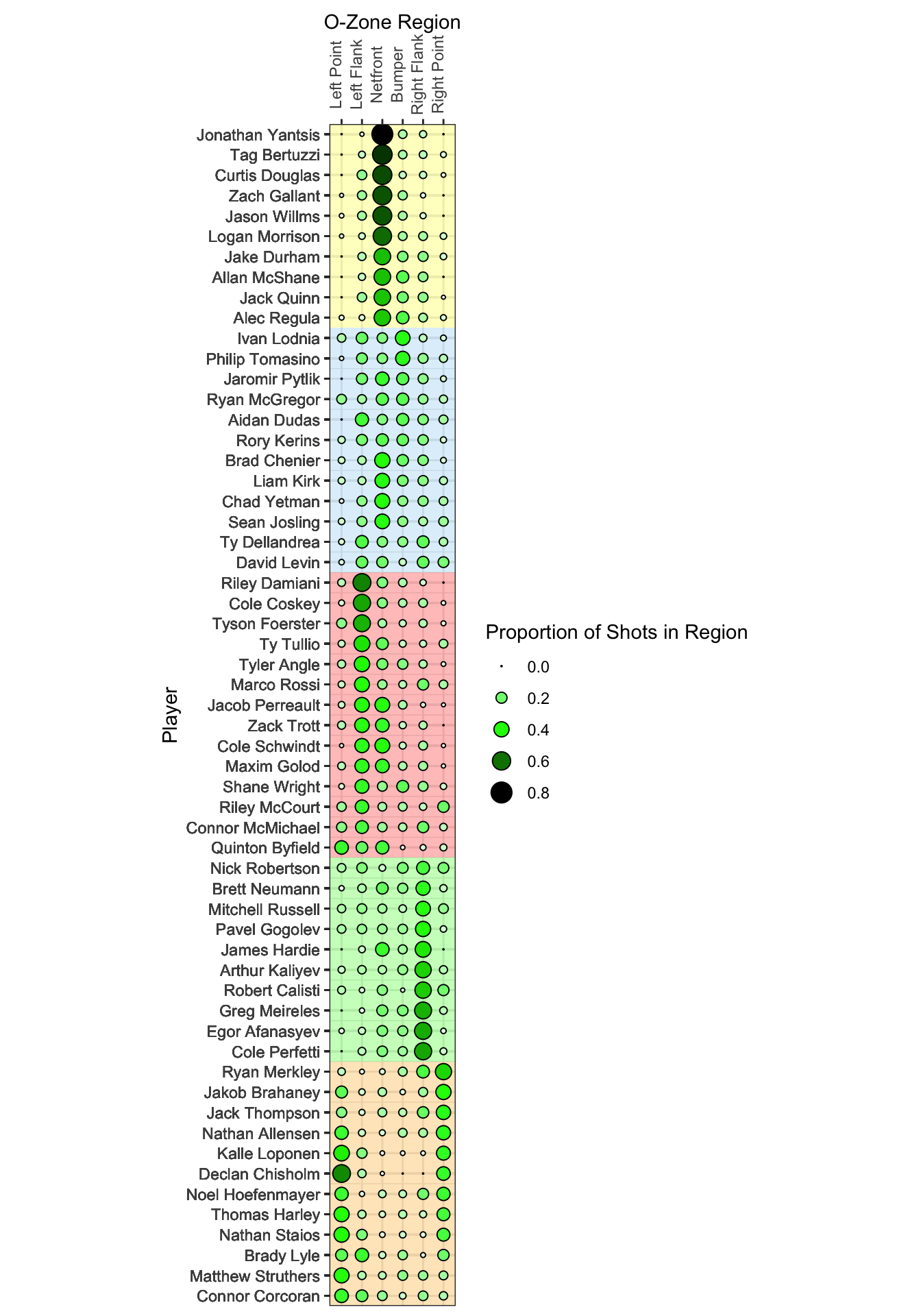
After cleaning up the data, I filtered for all OHLers with 40 or more PP shots leaving 58 players to analyze. Next, I binned each player's shots into six regions as displayed below. These regions represent the five traditional positions in an umbrella power play (netfront, bumper, left and right flank, point) with the point broken up into left and right sides to identify which side the pointman tends to lean on when shooting.
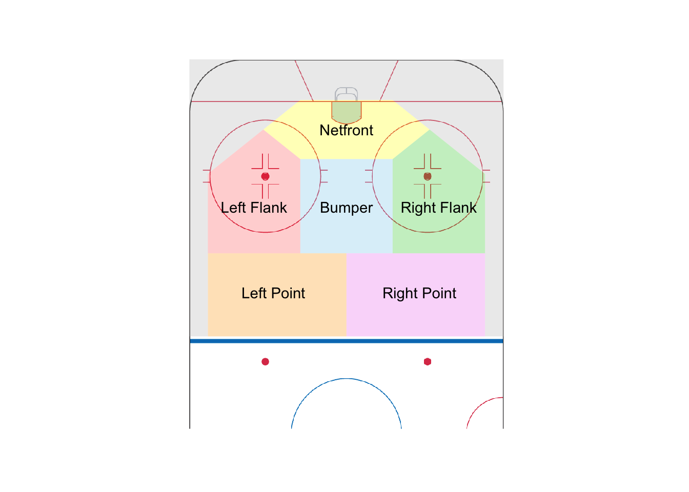
You might have also noticed the grey perimeter around these six regions. I was originally planning on including these shots into my analysis to identify any players who are taking an abundance of clearly low-danger shots, but no player in the data set had more than 5 shots from this region so I decided to chalk them up as noise and leave it out of the cluster analysis.
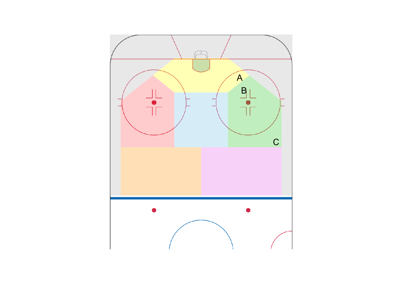
Binning the data is generally not preferred since it can lead to some similar shots being categorized differently and some different shots being treated as the same, especially with the small number of large bins used in this project. For example, in the figure below, we would treat shots A and B as completely different since they are in different regions, while B and C will be treated as the same since they both lie in the Right Flank region.
With that said, I believe binning is sufficient for clustering power play shot data due to the static nature of offensive teams on the PP and the consistency of the umbrella set up across nearly all levels of hockey. In addition, many of these players have a small sample size of shots (ranging from 40-114 SOG), so the large bin size may somewhat reduce the accuracy but will make the data easier to cluster.
(My next article will attempt to mitigate this binning issue and use a stronger clustering algorithm to solve this same problem with NHL even strength data. For now, this method works well on the OHL PP shot data and will provide a great visualization of the player shot tendencies, which I will display in the results section.)
Once I binned the data, I took the proportion of the player's total shots in each region. Taking the shot proportions rather than shot counts helps the clustering algorithm group players who are generating shots from similar areas, even if they have much different shot totals. For example, Arthur Kaliyev has 53 shots from the right flank region, accounting for 46.5% of his shots, while Egor Afanasyev has 29 shots from the right flank, which is 40.3% of his shots. Since we are more concerned in determining where players are shooting from rather than how much each player is shooting, proportions will provide better results.
That concludes the data preparation I did to setup the data for clustering. The following table is the first 6 rows of the final data frame I used for clustering.
| bumper | leftpoint | leftwing | netfront | rightpoint | rightwing | |
|---|---|---|---|---|---|---|
| Aidan Dudas | 0.2439 | 0.0000 | 0.2927 | 0.1707 | 0.1220 | 0.1707 |
| Alec Regula | 0.2609 | 0.0290 | 0.0435 | 0.4783 | 0.0435 | 0.1159 |
| Allan McShane | 0.2439 | 0.0000 | 0.0732 | 0.4878 | 0.0000 | 0.1463 |
| Arthur Kaliyev | 0.1491 | 0.0702 | 0.1053 | 0.1053 | 0.0965 | 0.4649 |
| Brad Chenier | 0.2128 | 0.0638 | 0.1064 | 0.4043 | 0.0426 | 0.1702 |
| Brady Lyle | 0.1389 | 0.2361 | 0.3056 | 0.0694 | 0.2083 | 0.0278 |
Fuzzy c-Means Clustering
As some of my Twitter followers may have seen, I also attempted to solve this same problem using Ward's method hierarchical clustering in the past. However, I opted to change to fuzzy c-means clustering (FCM) for this writeup because the flexible nature of its results is better-suited for the type of data I have.
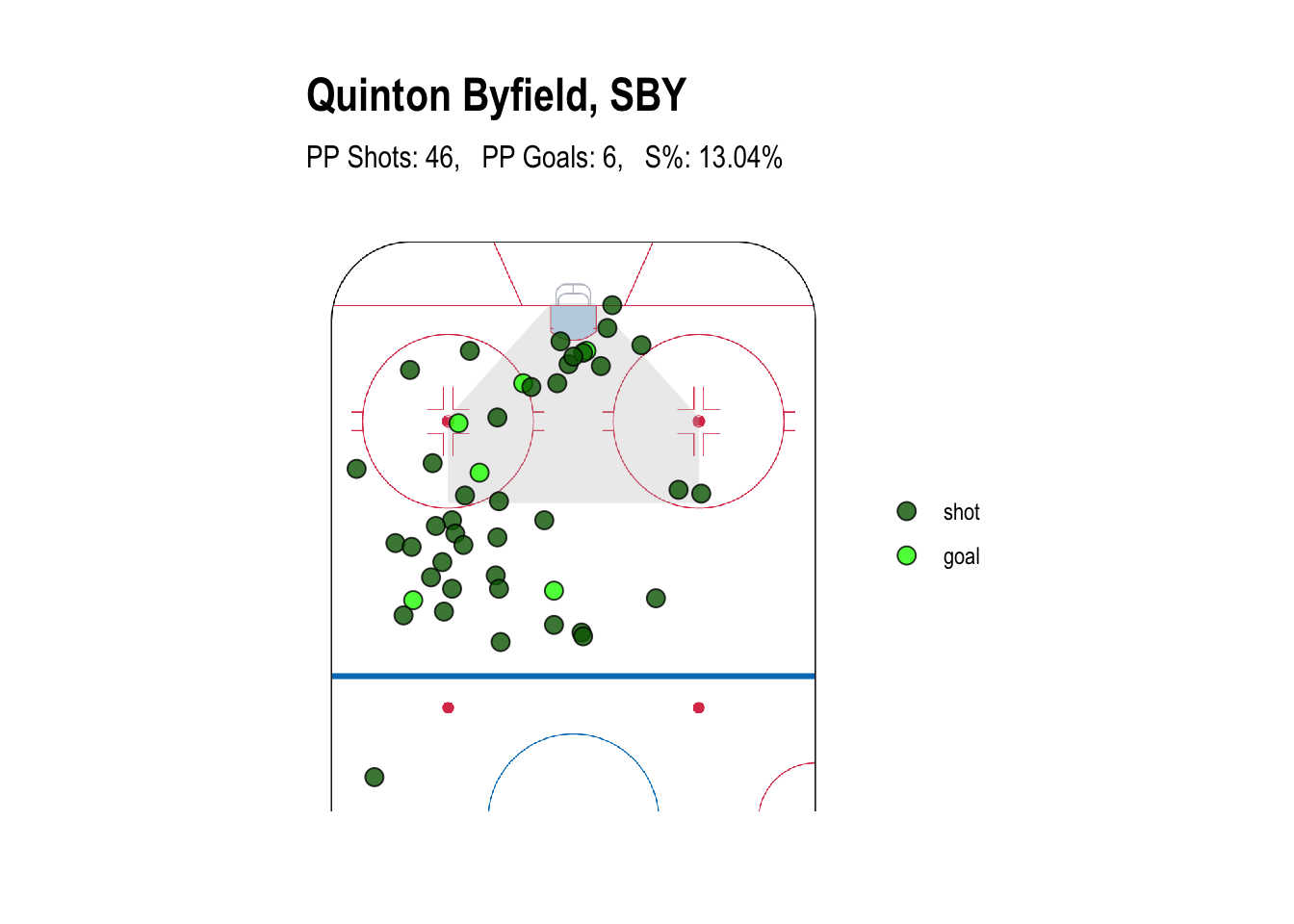
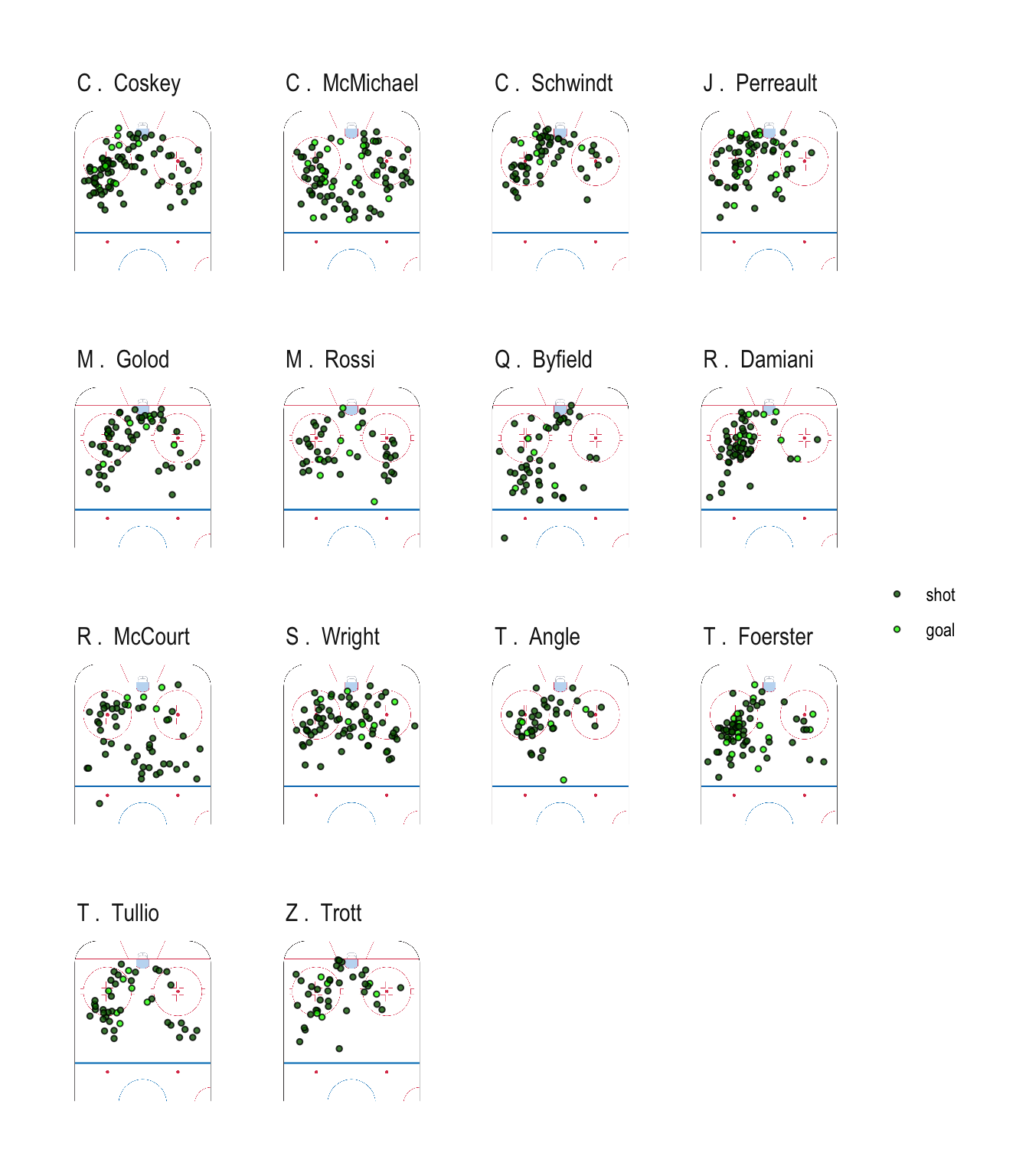
Fuzzy c-means is a "fuzzy" clustering algorithm, meaning that players are not strictly assigned to one cluster, but instead they are given a "degree" (between 0 and 1) to which they belong to each cluster. This feature is especially helpful when it comes to players that spent time at different spots on the power play over the season, whether that is caused by a trade or a coach trying to shake things up. For example, 2020 top prospect Quinton Byfield's PP shot chart below shows us that he has spent time this season both at the netfront and the left flank/left point. A method like hierarchical clustering will strictly define a player into one cluster, while fuzzy c-means allows Byfield to be in several different clusters to varying degrees.
Fuzzy c-Means Algorithm
Here is a simple overview of the steps that go into the fuzzy c-means algorithm:
Specify the number of clusters (5 clusters in hopes of finding 1 cluster for each PP position).
Randomly select 5 "cluster centres" (5 data points that are considered the average proportion of shots in each of the 6 regions for the players assigned to said cluster).
For each player, calculate the degree to which he belongs to each cluster.
Determine the "fuzzy" cluster centres that minimize the total weighted distance between each player and the cluster centres, where the weights are the degree to which a player belongs in the cluster.
Repeat 3 and 4 until you minimize the total weighted distance between each player and the fuzzy cluster centres.
If you were interested in learning more, I found this page helpful for understanding the math behind the FCM algorithm.
Clustering Results
The results of the FCM clustering are visualized below in a bubble heatmap. The background colour represents the 5 different clusters and the "bubbles" represent the proportion of shots in a given region for each player. It looks like the FCM algorithm does a pretty good job separating the five different PP positions.

Building off of this, I also plotted out the degree to which each player belongs to his designated cluster below. Players with low values (i.e. Byfield, Merkley, etc.) are not as tightly associated with their cluster and are more likely to have a high proportion of shots from multiple regions. On the other hand, players with high values (i.e. Wilms, Harley, etc.) have a very strong degree of association to their cluster and tend to have shots more focused in one region of the ice.
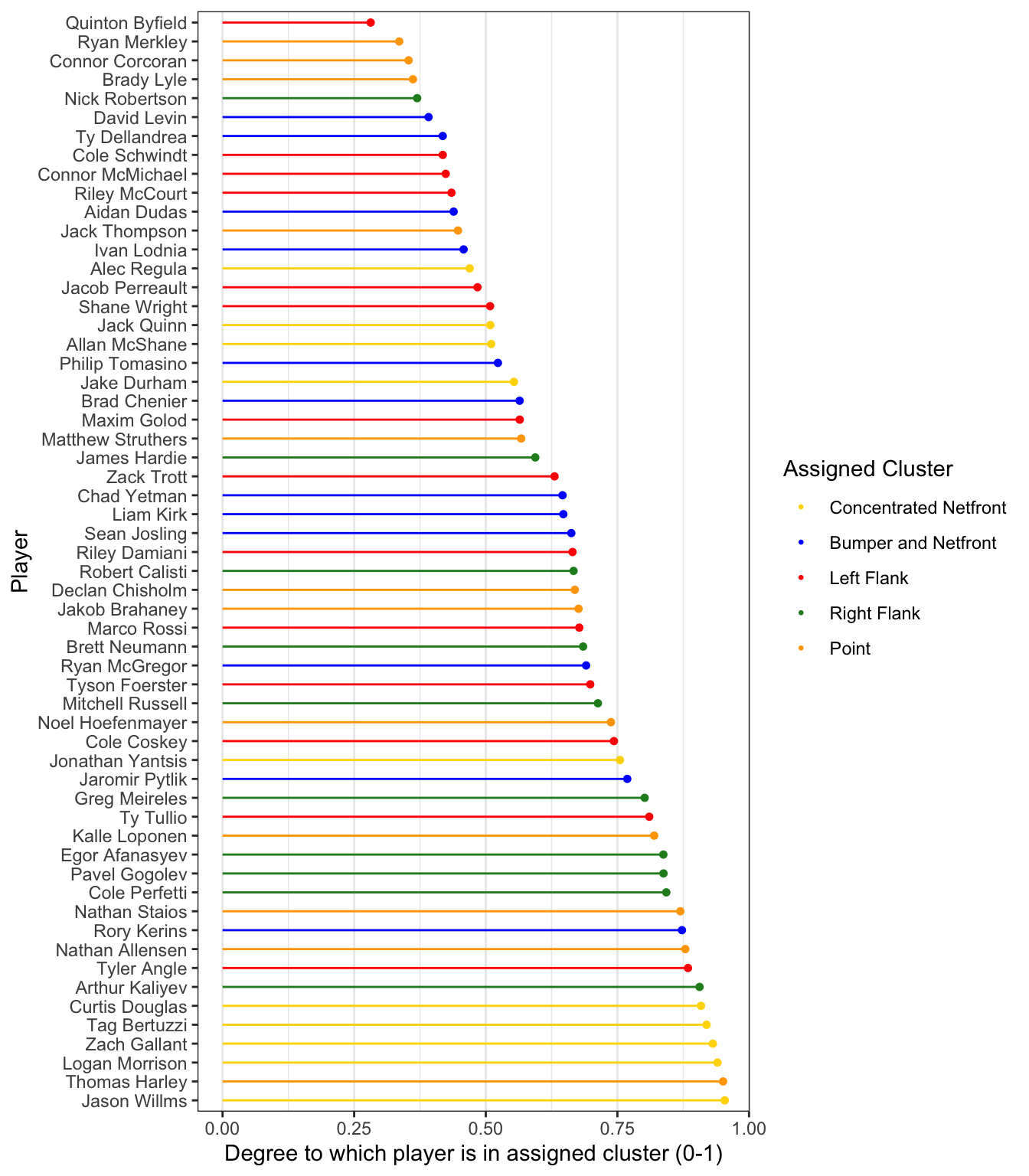
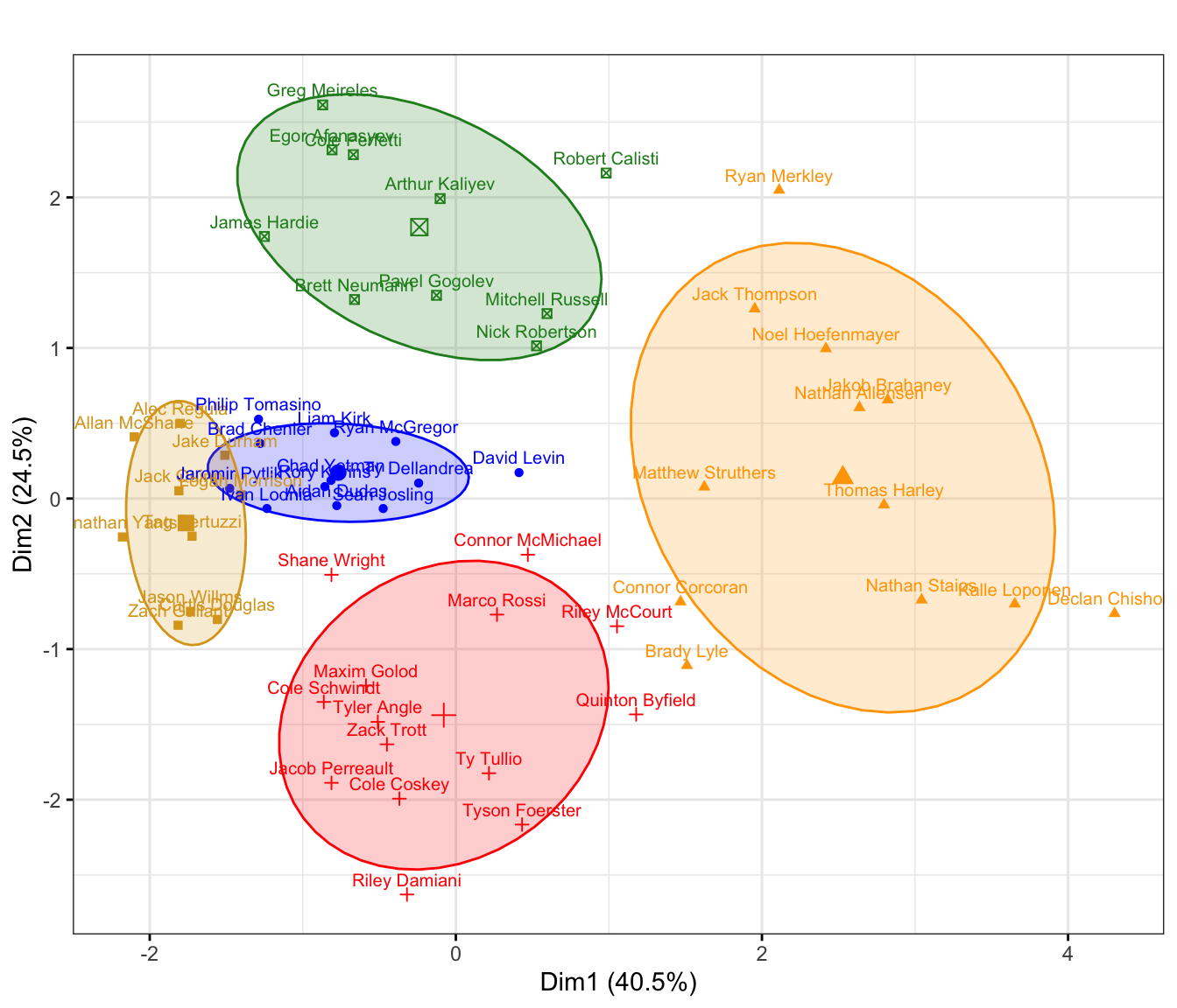
On top of that, I also visualized this data in 2D using Principal Component Analysis. This seems to reinforce the results of the degree of cluster membership plot above, with most players that have a low degree of cluster membership being on the fringes of their given cluster (i.e. Byfield, Merkley, Lyle, Levin, etc.).
There is also some overlap between the netfront (gold) and bumper (blue) clusters, which makes sense since bumper players tend to generate a good chunk of their shots from rebounds and scramble plays.
From a statistical perspective, it is also interesting to see that reducing the six-dimensional data matrix back to two dimensions generates a nearly exact image of where we would see on a 2D rink if we were to place each player based on their shot maps. The bumper (blue) is right behind the netfront (gold), the left (red) and right (green) flanks are to the left and right of the bumper (when facing the net), and the point (orange) is behind all of the other areas.

Now that we have an overview of the results, lets dig a little deeper into each of the five clusters.
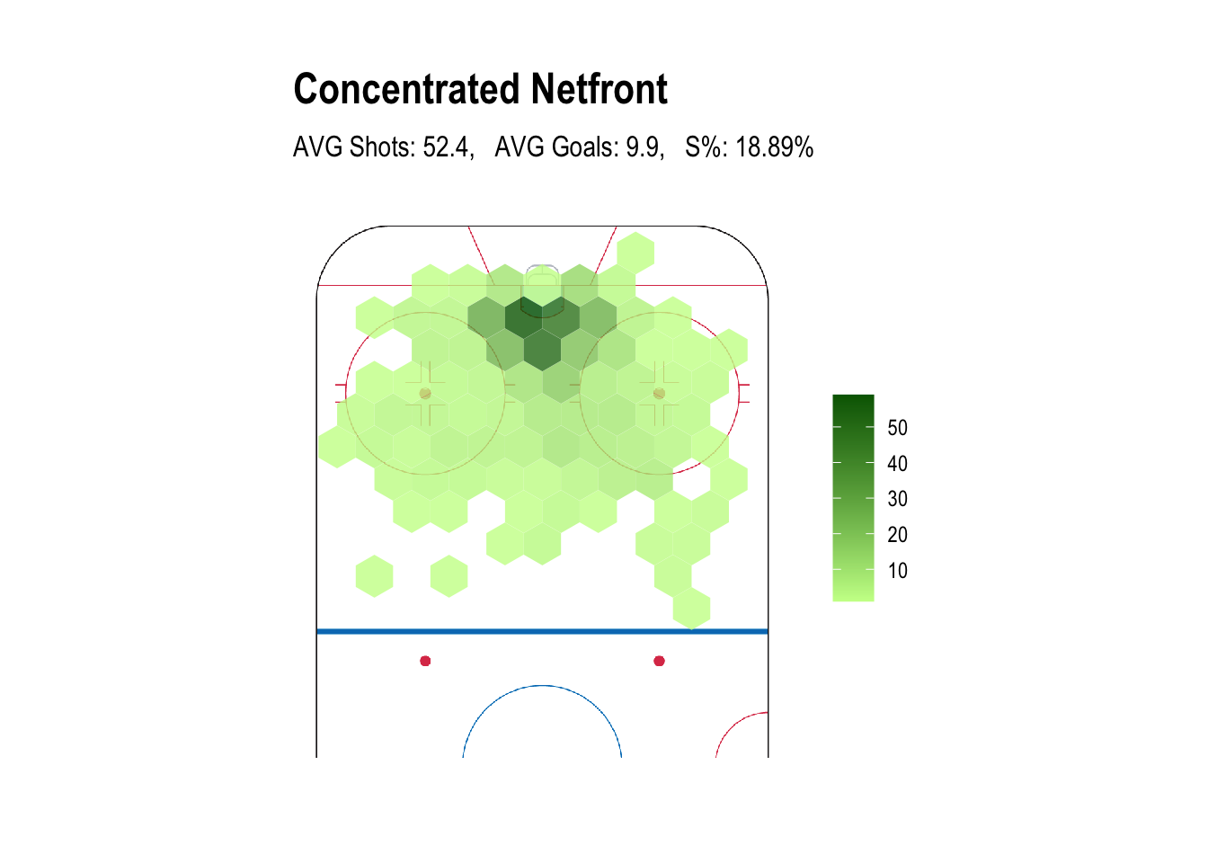
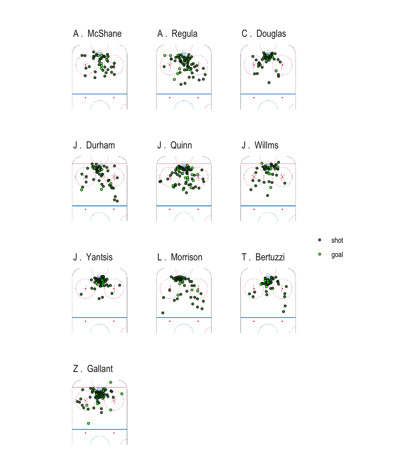
Cluster 1: Concentrated Netfront
The first cluster represents players that generate a very high proportion of their PP shots from the netfront as shown in the shot map below. They have the highest shooting percentage of all clusters with 18.89%, which may lead to a bit of inflation in their goal totals.
Interesting Observation: Alec Regula, the 6'4" London Knights' defenceman, is an odd player to find at the netfront. With Adam Boqvist/Evan Bouchard (18-19) and Merkley (19-20) already being excellent PP quarterbacks, the Knights decided to slide their big defenceman down low where he thrived in the netfront and bumper positions leading all defencemen with 15 PPG this season. However, this is something to consider when looking at his stats to project his offensive upside, 26 of his 60 points this season came on the PP and there is no guarantee that he will get PP time up front at the next level.
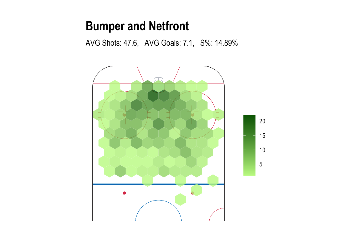
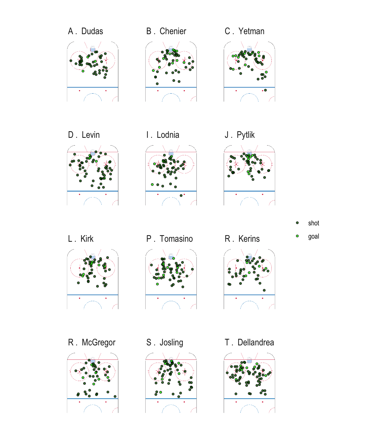
Cluster 2: Bumper and Netfront
This cluster somewhat corresponds to players in the bumper position. It is difficult to determine who actually plays in the bumper spot based on PP shot charts alone since penalty killers tend to smother this area making chances here few and far between. They are used as a decoy to some degree, keeping the PK in the box formation, which opens up the flanks and point. Many of their touches end in quick passes to a player with more time and space. Most players here produce as many netfront shots as bumper shots from crashing the net for rebounds.
Interesting Observation: Phil Tomasino and Ivan Lodnia lead the league in percentage of shots from the bumper region (34.6% and 37.0%, respectively). This is no small feat considering how heavily-guarded the middle of the ice is on the PP.
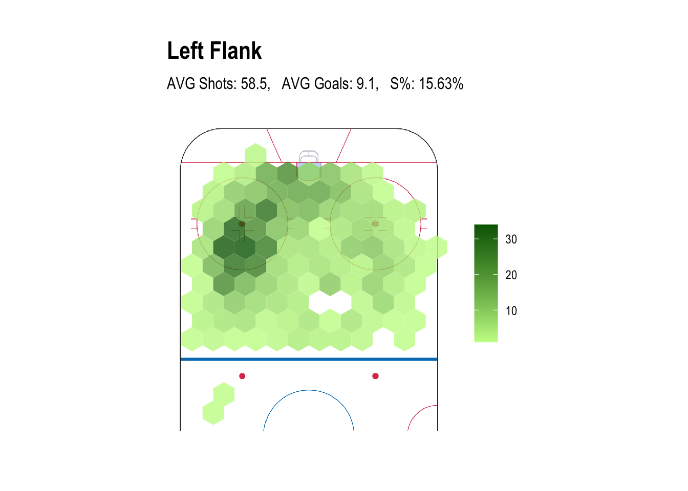
Cluster 3: Left Flank
These players hang out in the upper left circle moving the puck around between the point and the right flank in hopes of generating a strong one-time chance with pre-shot movement. This pre-shot movement along with the time and space they are afforded due to penalty killers generally collapsing into a box to protect the slot gives this position a high 15.63 S% despite the long distance and bad angle from the net.
Interesting Observation: 2020 draft eligible forward Tyson Foerster is a standout here due to his ridiculously high volume of shots from the upper left circle. The quantity of shots from this area (most of which are likely one-timers) combined with his lethal slapshot led him to an OHL-leading 18 PPG this season. These shades of Ovi make him an interesting prospect in this year's draft.
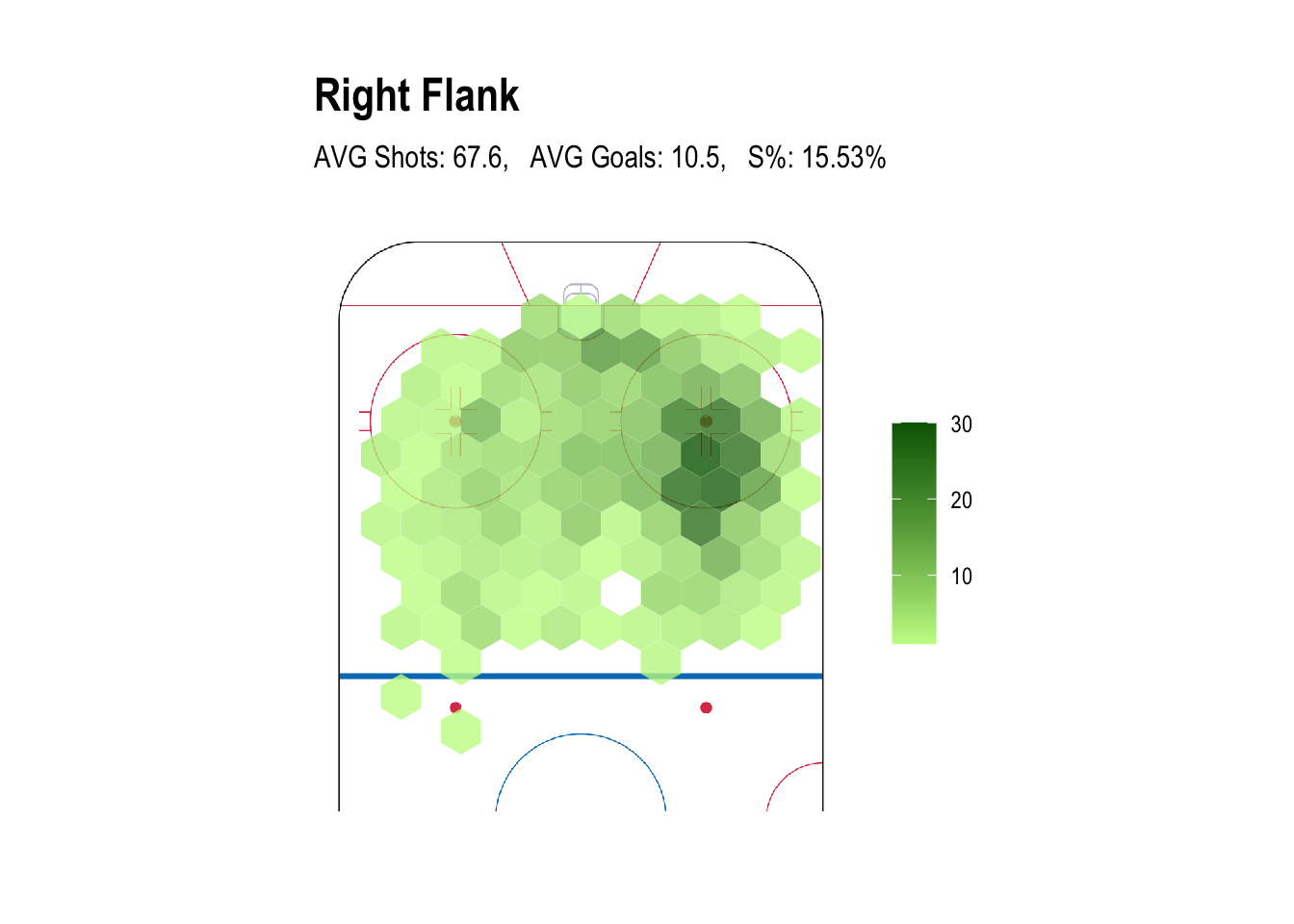
Cluster 4: Right Flank
Same as the left flank, just on the right side.
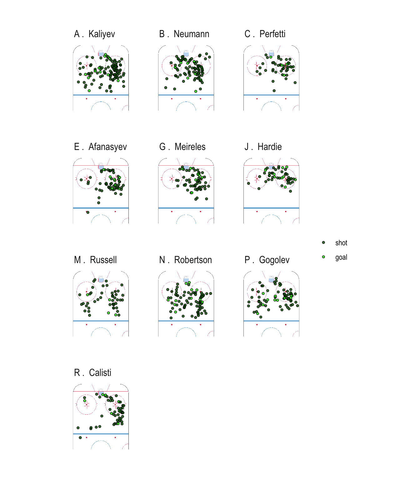
Interesting Observation: Two of the most lethal goal scorers in the OHL, Arthur Kaliyev and Nick Robertson, fall into the right flank cluster. Kaliyev (16 PPG) and Robertson (13 PPG) are excellent one-time threats on the right side, but their shot maps show that they are not as static as Tyson Foerster is on the left, they both finds ways to generate shots from all over the offensive zone making them more dynamic scorers.
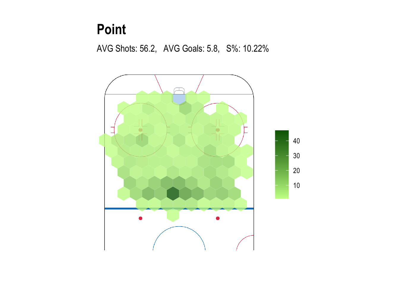
Cluster 5: The Point
This cluster consists of the PP "Quarterbacks" who spend a lot of time controlling the puck and trying to manipulate penalty killers so they can open up a one-time chance for their flanks. Due to the distance from the net, they tend to have a lower shooting percentage and, in turn, a lower goal total.
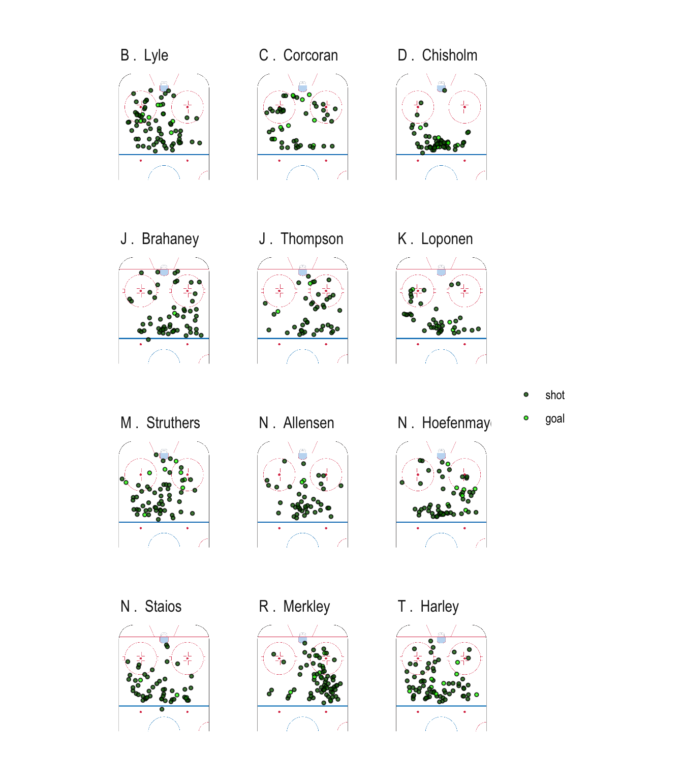
Interesting Observation: Playing the opposite role of Alec Regula at the netfront, Matthew Struthers is the lone forward among this group of PP QBs. He started the season playing the PP point role in North Bay and was traded to Owen Sound midseason where they ended up sliding their QB Brady Lyle to the left flank to open up room for Struthers at the point.
Cluster Summary
| Cluster | Avg Shots | Avg Goals | Shooting % | Notable Players |
|---|---|---|---|---|
| Concentrated Netfront | 52.4 | 9.9 | 18.89% | Jack Quinn (2020), Alec Regula (CHI) |
| Bumper and Netfront | 47.6 | 7.1 | 14.89% | Phil Tomasino (NSH), Ty Dellandrea (DAL) |
| Left Flank | 58.5 | 9.1 | 15.63% | Shane Wright (2022), Connor McMichael (WSH), Quinton Byfield (2020), Marco Rossi (2020) |
| Right Flank | 67.6 | 10.5 | 15.53% | Nick Robertson (TOR), Arthur Kaliyev (LA), Cole Perfetti (2020) |
| The Point | 56.2 | 5.8 | 10.22% | Thomas Harley (DAL), Ryan Merkley (SJ) |
Conclusion
This approach was specifically meant for power play shot data with a small sample and, as I mentioned at the beginning, there are some clear limitations of my methodology:
The large bin sizes leads to a loss of information in the data, which makes it difficult to separate more subtle differences between shot maps. For this reason, it would be difficult to cluster even strength shot data using this method.
Clustering players by PP shots tells us more about where a coach is placing a player on the PP rather than actually gaining any insights about the player's style of play.
With that being said, I think this method did a good job identifying PP positions through clustering. I hope that casual fans were able to see where their team's top prospects are generating shots on the power play and that analytics nerds have gained some new tools that may be applied in other ways in the future.
If you had any questions, comments, or concerns or wanted to see any OHL player's shot chart at any strength state, feel free to tweet me @ BrendanKumagai or email me at brendankumagai@gmail.com.
The Code
Loading the Data and Packages
Load all necessary packages.
library(tidyverse) # For various data science packages

library(png) # For loading in png's

library(gcookbook); library(hrbrthemes) # For theme_ipsum() in ggplot

library(sp) # For binning shots

library(reshape2) # For the melt() and dcast() functions

library(plotly) # To make interactive plots

library(magrittr) # For the set_rownames() function

library(ggalt) # For making lollipop charts

library(e1071) # For fuzzy c-means clustering

library(factoextra) # For visualizing the data using PCA

library(ggnewscale) # For setting multiple fill scales in ggplot

library(ggalt) # For lollipop charts
Load the data set (this data can be found on my Github under content/article/projectdata) and the png of the half rink.
# Load the OHL shot data
ohl.shot.data = read_csv("projectdata/ohl-shot-data.csv")

# Load the half rink png
halfrink = readPNG("projectpics/nhlhalfrink.png")
Preparing and Binning the Data
Create the different regions of the offensive zone that we will use for clustering. Each of the regions below are represented by a data frame that contains the xy-coordinates of a polygon that encloses that region.
netfront = data.frame("x" = c(-12.5, -22.5, -12.5, 12.5, 22.5, 12.5), "y" = c(89, 81, 73, 73, 81, 89))

bumper = data.frame("x" = c(-12.5, -12.5, 12.5, 12.5), "y" = c(73, 47.5, 47.5, 73))

leftwing = data.frame("x" = c(-37.5, -37.5, -22.5, -12.5, -12.5), "y" = c(47.5, 69, 81, 73, 47.5))

rightwing = data.frame("x" = c(37.5, 37.5, 22.5, 12.5, 12.5), "y" = c(47.5, 69, 81, 73, 47.5))

leftpoint = data.frame("x" = c(-37.5, -37.5, 0, 0), "y" = c(47.5, 25, 25, 47.5))

rightpoint = data.frame("x" = c(0, 0, 37.5, 37.5), "y" = c(47.5, 25, 25, 47.5))

perimeter = data.frame("x" = c(-42.5, -42.5, 42.5, 42.5, 37.5, 37.5, 12.5, -12.5, -37.5, -37.5),
                       "y" = c(25, 100, 100, 25, 25, 69, 89, 89, 69, 25))
Plot the different regions that the data is to be binned into.
# Create a ggplot with data = data.frame(0) since we won't be using any data to make it
ggplot(data = data.frame(0)) +
    # Use theme ipsum
    theme_ipsum(axis_text_size = 0, grid = FALSE) +
    # Add in the rink plot
    annotation_raster(halfrink, ymin = 0, ymax= 100, xmin = -42.5, xmax = 42.5) +
    # Add in the shading for each region
    geom_polygon(data = netfront, aes(x = x, y = y), fill = "yellow", alpha = 0.3) +
    geom_polygon(data = bumper, aes(x = x, y = y), fill = "skyblue", alpha = 0.3) +
    geom_polygon(data = leftpoint, aes(x = x, y = y), fill = "orange", alpha = 0.3) +
    geom_polygon(data = rightpoint, aes(x = x, y = y), fill = "violet", alpha = 0.3) +
    geom_polygon(data = perimeter, aes(x = x, y = y), fill = "grey", alpha = 0.3) +
    geom_polygon(data = leftwing, aes(x = x, y = y), fill = "red", alpha = 0.2) +
    geom_polygon(data = rightwing, aes(x = x, y = y), fill = "limegreen", alpha = 0.3) +
    # Add in labels for each region
    geom_text(x = 0, y = 81, label = "Netfront") +
    geom_text(x = 0, y = 60, label = "Bumper") +
    geom_text(x = 25, y = 60, label = "Right Flank") +
    geom_text(x = -25, y = 60, label = "Left Flank") +
    geom_text(x = 19.75, y = 36.875, label = "Right Point") +
    geom_text(x = -19.75, y = 36.875, label = "Left Point") +
    # Limit the xy-coordinate range to just the rink
    lims(x = c(-42.5, 42.5), y = c(0, 100)) +
    # Set the aspect ratio at 1
    coord_fixed(ratio = 1) +
    # Remove all labels
    labs(x = NULL, y = NULL)

Now that the regions are defined, bin the shot data for each player into these 7 regions then remove the perimeter region. Following that, calculate the proportion of shots in each region.
# Calculate the total number of shots in each region for each player
ohl.pp.region.counts = ohl.shot.data %>%
  # Select just PP shots
  filter(strength == "PP") %>%
  # Create categorical variables for each region that are 1 if the shot is in the specified
  # region and 0 if not using the point.in.polygon function
  mutate(netfront = point.in.polygon(real_x, real_y, netfront$x, netfront$y),
         bumper = point.in.polygon(real_x, real_y, bumper$x, bumper$y),
         leftpoint = point.in.polygon(real_x, real_y, leftpoint$x, leftpoint$y),
         rightpoint = point.in.polygon(real_x, real_y, rightpoint$x, rightpoint$y),
         perimeter = point.in.polygon(real_x, real_y, perimeter$x, perimeter$y),
         leftwing = point.in.polygon(real_x, real_y, leftwing$x, leftwing$y),
         rightwing = point.in.polygon(real_x, real_y, rightwing$x, rightwing$y)) %>%
  # The point.in.polygon function labels regions as 2 if they are on the edge of the region
  # Reduce all of these instances from 2 to 1
  mutate(netfront = ifelse(netfront == 2, 1, netfront),
         bumper = ifelse(bumper == 2, 1, bumper),
         leftpoint = ifelse(leftpoint == 2, 1, leftpoint),
         rightpoint = ifelse(rightpoint == 2, 1, rightpoint),
         perimeter = ifelse(perimeter == 2, 1, perimeter),
         leftwing = ifelse(leftwing == 2, 1, leftwing),
         rightwing = ifelse(rightwing == 2, 1, rightwing)) %>%
  # Calculate the sum of each of the regions (should be 1 for all shots)
  mutate(sum = netfront + bumper + leftpoint + rightpoint + perimeter + leftwing + rightwing) %>%
  # Reduce shots that are classified as multiple regions (on the edge of 2 regions) down to 1
  mutate(perimeter = ifelse(perimeter == 1 & sum == 2, 0, perimeter),
         leftpoint = ifelse(leftpoint == 1 & rightpoint == 1, 0, leftpoint),
         leftpoint = ifelse(leftpoint == 1 & leftwing == 1, 0, leftpoint),
         rightpoint = ifelse(rightpoint == 1 & rightwing == 1, 0, rightpoint),
         bumper = ifelse(bumper == 1 & sum == 2, 0, bumper),
         netfront = ifelse(netfront == 1 & leftwing == 1, 0, netfront),
         netfront = ifelse(netfront == 1 & rightwing == 1, 0, netfront)) %>%
  # Recalculate the sum
  mutate(sum2 = netfront + bumper + leftpoint + rightpoint + perimeter + leftwing + rightwing) %>%
  # Remove all shots that are not in a region (outside of the blue line)
  filter(sum2 != 0) %>%
  # Select only the player column and the column for each region
  select(player, netfront, bumper, leftpoint, rightpoint, perimeter, leftwing, rightwing) %>%
  # Create a column called "region" that represents which region the shot came from
  mutate(region = case_when(
    netfront == 1 ~ "netfront",
    bumper == 1 ~ "bumper",
    leftpoint == 1 ~ "leftpoint",
    rightpoint == 1 ~ "rightpoint",
    perimeter == 1 ~ "perimeter",
    leftwing == 1 ~ "leftwing",
    rightwing == 1 ~ "rightwing"
  )) %>%
  # Tally the amount of shots each player has in each region
  group_by(player, region) %>%
  tally() %>%
  # "Widen" the data to have one column for each region again but with each row
  # representing a player rather than a shot
  dcast(player ~ region, value.var = "n") %>%
  # Replace all NA's with 0
  replace(is.na(.), 0) %>%
  # Filter for players with only 40+ shots
  filter(bumper + leftpoint + rightpoint + leftwing + rightwing + netfront + perimeter >= 40)

# Calculate the proportion of shots in each region for each player
ohl.pp.region.proportions = ohl.pp.region.counts %>%
  # Find each player's total shots
  mutate(sum = leftwing + rightwing + leftpoint + rightpoint + netfront + bumper + perimeter) %>%
  # Calculate the proportion of shots in each region
  mutate(leftwing = leftwing / sum, rightwing = rightwing / sum,
         leftpoint = leftpoint / sum, rightpoint = rightpoint / sum,
         netfront = netfront / sum, bumper = bumper / sum) %>%
  # Remove the perimeter and sum columns (useless needed for clustering)
  select(-perimeter, -sum) %>%
  # Turn the player column into the row names
  column_to_rownames("player")
Performing fuzzy c-means clustering on the data
With the data processing complete, perform fuzzy c-means clustering on the data and add the results to the binned data frame and the complete shot data.
# Set a seed so the results can be recreated
set.seed(262626)

# Perform fuzzy c-means on the data with 5 clusters
ohl.pp.region.FCM = cmeans(ohl.pp.region.proportions, 5, m = 2)

# Create a data frame with the degrees of cluster membership
ohl.pp.region.FCM.memb = ohl.pp.region.FCM$membership %>%
  data.frame() %>%
  # Move player names from rownames to their own column
  rownames_to_column("player") %>%
  # Determine the max degree of membership (for future use)
  mutate(max = pmax(X1, X2, X3, X4, X5)) %>%
  # Rename the clusters
  rename("Bumper and Netfront" = "X1", "Point" = "X2", "Concentrated Netfront" = "X3", "Left Flank" = "X4", "Right Flank" = "X5")

# Add the cluster labels to the binned proportion data
ohl.pp.region.clusters = ohl.pp.region.proportions %>%
  # Move player names from rownames to their own column
  rownames_to_column("player") %>%
  # Add in the cluster
  mutate(cluster = factor(ohl.pp.region.FCM$cluster, levels = c(3,1,4,5,2),
                          labels = c("Concentrated Netfront", "Bumper and Netfront", "Left Flank", "Right Flank", "Point")))

# Add the player cluster label the shot data
ohl.shot.data = ohl.shot.data %>%
  # Match the cluster label to the player name
  mutate(player_cluster = ohl.pp.region.clusters$cluster[match(player, ohl.pp.region.clusters$player)])
Creating the shot plots
Create a function that makes it simple to create a shot plot.
# Create the function (choose subject = "playerfirstname playerlastname" or clust = "cluster label")
shot.plots = function(data = ohl.shot.data, subject = NULL, clust = NULL, all = TRUE, es = TRUE, pp = TRUE, sh = TRUE) {

  # Load in required packages
  library(tidyverse)
  library(png)
  library(gcookbook)
  library(hrbrthemes)

  # Load in half rink image
  halfrink = readPNG("projectpics/nhlhalfrink.png")

  # Create a polygon representing the homeplate
  homeplate = data.frame("x" = c(-4, -22, -22, 22, 22, 4), "y" = c(89, 69, 54, 54, 69, 89))

  # If we want a player's shot map use this
  if (!is.null(subject)) {
    ohl.run = data %>%
      filter(player == subject)

    # Plot all of the player's shots
    gg1 = ggplot(ohl.run) +
      theme_ipsum(axis_text_size = 0, grid = FALSE) +
      annotation_raster(halfrink, ymin = 0, ymax= 100, xmin = -42.5, xmax = 42.5) +
      geom_polygon(data = homeplate, aes(x = x, y = y), fill = "grey", alpha = 0.3) +
      geom_point(aes(x = real_x, y = real_y, fill = factor(strength, levels = c("ES", "PP", "SH"))), size = 3, shape = 21, alpha = 0.8) +
      lims(x = c(-42.5, 42.5), y = c(0,100)) +
      scale_fill_manual(values = c("blue", "green", "red")) +
      coord_fixed(ratio = 1) +
      labs(title = paste(ohl.run$player[1], ", ", ohl.run$off_team[nrow(ohl.run)], sep = ""),
           subtitle = paste("Total Shots: ", nrow(ohl.run), ",   Total Goals: ", nrow(ohl.run %>% filter(event == "goal")),
                            ",   S%: ", 100*round(nrow(ohl.run %>% filter(event == "goal"))/nrow(ohl.run), 4), "%", sep = ""),
           x = NULL, y = NULL, fill = "Strength")

    # Plot ES shots
    gg2 = ggplot(ohl.run %>% filter(strength == "ES")) +
      theme_ipsum(axis_text_size = 0, grid = FALSE) +
      annotation_raster(halfrink, ymin = 0, ymax= 100, xmin = -42.5, xmax = 42.5) +
      geom_polygon(data = homeplate, aes(x = x, y = y), fill = "grey", alpha = 0.3) +
      geom_point(aes(x = real_x, y = real_y, fill = factor(event, levels = c("shot", "goal"))), size = 3, shape = 21, alpha = 0.8) +
      lims(x = c(-42.5, 42.5), y = c(0,100)) +
      scale_fill_manual(values = c("navy", "skyblue")) +
      coord_fixed(ratio = 1) +
      labs(title = paste(ohl.run$player[1], ", ", ohl.run$off_team[nrow(ohl.run)], sep = ""),
           subtitle = paste("ES Shots: ", nrow(ohl.run %>% filter(strength == "ES")), ",   ES Goals: ", nrow(ohl.run %>% filter(event == "goal", strength == "ES")),
                            ",   S%: ", 100*round(nrow(ohl.run %>% filter(event == "goal", strength == "ES"))/nrow(ohl.run %>% filter(strength == "ES")), 4), "%", sep = ""),
           x = NULL, y = NULL, fill = NULL)

    # Plot PP shots
    gg3 = ggplot(ohl.run %>% filter(strength == "PP")) +
      theme_ipsum(axis_text_size = 0, grid = FALSE) +
      annotation_raster(halfrink, ymin = 0, ymax= 100, xmin = -42.5, xmax = 42.5) +
      geom_polygon(data = homeplate, aes(x = x, y = y), fill = "grey", alpha = 0.3) +
      geom_point(aes(x = real_x, y = real_y, fill = factor(event, levels = c("shot", "goal"))), size = 3, shape = 21, alpha = 0.8) +
      lims(x = c(-42.5, 42.5), y = c(0,100)) +
      scale_fill_manual(values = c("darkgreen", "green")) +
      coord_fixed(ratio = 1) +
      labs(title = paste(ohl.run$player[1], ", ", ohl.run$off_team[nrow(ohl.run)], sep = ""),
           subtitle = paste("PP Shots: ", nrow(ohl.run %>% filter(strength == "PP")), ",   PP Goals: ", nrow(ohl.run %>% filter(event == "goal", strength == "PP")),
                            ",   S%: ", 100*round(nrow(ohl.run %>% filter(event == "goal", strength == "PP"))/nrow(ohl.run %>% filter(strength == "PP")), 4), "%", sep = ""),
           x = NULL, y = NULL, fill = NULL)

    # Plot SH shots
    gg4 = ggplot(ohl.run %>% filter(strength == "SH")) +
      theme_ipsum(axis_text_size = 0, grid = FALSE) +
      annotation_raster(halfrink, ymin = 0, ymax= 100, xmin = -42.5, xmax = 42.5) +
      geom_polygon(data = homeplate, aes(x = x, y = y), fill = "grey", alpha = 0.3) +
      geom_point(aes(x = real_x, y = real_y, fill = factor(event, levels = c("shot", "goal"))), size = 3, shape = 21, alpha = 0.8) +
      lims(x = c(-42.5, 42.5), y = c(0,100)) +
      scale_fill_manual(values = c("darkred", "firebrick1")) +
      coord_fixed(ratio = 1) +
      labs(title = paste(ohl.run$player[1], ", ", ohl.run$off_team[nrow(ohl.run)], sep = ""),
           subtitle = paste("SH Shots: ", nrow(ohl.run %>% filter(strength == "SH")), ",   SH Goals: ", nrow(ohl.run %>% filter(event == "goal", strength == "SH")),
                            ",   S%: ", 100*round(nrow(ohl.run %>% filter(event == "goal", strength == "SH"))/nrow(ohl.run %>% filter(strength == "SH")), 4), "%", sep = ""),
           x = NULL, y = NULL, fill = NULL)
  }

  # If we want a cluster's shot heatmap use this
  if (!is.null(clust)) {
    ohl.run = data %>%
      filter(player_cluster == clust)

    # Create a hexbin plot of all shots from all players in cluster
    gg1 = ggplot(ohl.run) +
      theme_ipsum(axis_text_size = 0, grid = FALSE) +
      annotation_raster(halfrink, ymin = 0, ymax= 100, xmin = -42.5, xmax = 42.5) +
      geom_hex(aes(x = real_x, y = real_y), alpha = 0.8, binwidth = 7) +
      lims(x = c(-42.5, 42.5), y = c(0,100)) +
      scale_fill_gradient2(low = "white", mid = "grey45", high = "black") +
      coord_fixed(ratio = 1) +
      labs(title = clust,
           subtitle = paste("Total Shots: ", nrow(ohl.run), ", Total Goals: ", nrow(ohl.run %>% filter(event == "goal")), sep = ""),
           x = NULL, y = NULL, fill = "Strength")

    # Create a hexbin plot of ES shots from all players in cluster
    gg2 = ggplot(ohl.run %>% filter(strength == "ES")) +
      theme_ipsum(axis_text_size = 0, grid = FALSE) +
      annotation_raster(halfrink, ymin = 0, ymax= 100, xmin = -42.5, xmax = 42.5) +
      geom_hex(aes(x = real_x, y = real_y), alpha = 0.8, binwidth = 7) +
      scale_fill_gradient2(low = "white", mid = "skyblue", high = "navy") +
      lims(x = c(-42.5, 42.5), y = c(0,100)) +
      coord_fixed(ratio = 1) +
      labs(title = clust,
           subtitle = paste("ES Shots: ", nrow(ohl.run %>% filter(strength == "ES")), ", ES Goals: ", nrow(ohl.run %>% filter(event == "goal", strength == "ES")), sep = ""),
           x = NULL, y = NULL, fill = NULL)

    # Create a hexbin plot of PP shots from all players in cluster
    gg3 = ggplot(ohl.run %>% filter(strength == "PP")) +
      theme_ipsum(axis_text_size = 0, grid = FALSE) +
      annotation_raster(halfrink, ymin = 0, ymax= 100, xmin = -42.5, xmax = 42.5) +
      geom_hex(aes(x = real_x, y = real_y), alpha = 0.8, binwidth = 7) +
      lims(x = c(-42.5, 42.5), y = c(0,100)) +
      scale_fill_gradient2(low = "white", mid = "#CCFF99", high = "darkgreen") +
      # scale_fill_manual(values = c("darkgreen", "green")) +
      coord_fixed(ratio = 1) +
      labs(title = clust,
           subtitle = paste("AVG Shots: ", round(nrow(ohl.run %>% filter(strength == "PP"))/nrow(ohl.pp.region.clusters %>% filter(cluster == clust)), 1),
                            ",   AVG Goals: ", round(nrow(ohl.run %>% filter(event == "goal", strength == "PP")) /
                                                     nrow(ohl.pp.region.clusters %>% filter(cluster == clust)), 1),
                            ",   S%: ", round(nrow(ohl.run %>% filter(event == "goal", strength == "PP"))/nrow(ohl.run %>% filter(strength == "PP")), 4) * 100, "%", sep = ""),
           x = NULL, y = NULL, fill = NULL)

    # Create a hexbin plot of SH shots from all players in cluster
    gg4 = ggplot(ohl.run %>% filter(strength == "SH")) +
      theme_ipsum(axis_text_size = 0, grid = FALSE) +
      annotation_raster(halfrink, ymin = 0, ymax= 100, xmin = -42.5, xmax = 42.5) +
      geom_hex(aes(x = real_x, y = real_y), alpha = 0.8, binwidth = 7) +
      scale_fill_gradient2(low = "white", mid = "white", high = "maroon") +
      lims(x = c(-42.5, 42.5), y = c(0,100)) +
      coord_fixed(ratio = 1) +
      labs(title = clust,
           subtitle = paste("SH Shots: ", nrow(ohl.run %>% filter(strength == "SH")), ", SH Goals: ", nrow(ohl.run %>% filter(event == "goal", strength == "SH")), sep = ""),
           x = NULL, y = NULL, fill = NULL)
  }

  # Print whichever ones you selected as true
  if (all == TRUE) {print(gg1)}

  if (es == TRUE) {print(gg2)}

  if (pp == TRUE) {print(gg3)}

  if (sh == TRUE) {print(gg4)}
}
Visualizing the cluster results
Visualize the cluster results in a bubble heatmap.
# Select and order concentrated netfront cluster players
nf.order = ohl.pp.region.clusters %>%
  filter(cluster == "Concentrated Netfront") %>%
  arrange(netfront) %>%
  select(player) %>%
  unlist()

# Select and order bumper and netfront cluster players
bp.order = ohl.pp.region.clusters %>%
  filter(cluster == "Bumper and Netfront") %>%
  arrange(bumper) %>%
  select(player) %>%
  unlist()

# Select and order left flank cluster players
lf.order = ohl.pp.region.clusters %>%
  filter(cluster == "Left Flank") %>%
  arrange(leftwing) %>%
  select(player) %>%
  unlist()

# Select and order right flank cluster players
rf.order = ohl.pp.region.clusters %>%
  filter(cluster == "Right Flank") %>%
  arrange(desc(rightwing)) %>%
  select(player) %>%
  unlist()

# Select and order point cluster players
pt.order = ohl.pp.region.clusters %>%
  filter(cluster == "Point") %>%
  arrange(rightpoint) %>%
  select(player) %>%
  unlist()

# Combine all five of the clusters to get the order desired for the bubble heatmap
ohl.order = c(pt.order, rf.order, lf.order, bp.order, nf.order)

# Create a data frame for ggplot to the bubble heatmap off of
ohl.pp.region.bheat = ohl.pp.region.proportions %>%
  # Move the player names from the rownames to their own column
  rownames_to_column("player") %>%
  # Reformat the data so there are 3 columns (player, region, proportion) and each player has 6 rows (one for each region)
  melt(id.vars = "player", variable.name = "region", value.name = "proportion") %>%
  # Add in the cluster as determined by fuzzy c-means
  mutate(cluster = ohl.pp.region.clusters$cluster[match(player, ohl.pp.region.clusters$player)]) %>%
  # Turn the player column into a factor so we can order it based on cluster
  mutate(player = factor(player, levels = ohl.order)) %>%
  # Create a dummy variable Y that will be used in ggplot
  mutate(Y = as.numeric(player)) %>%
  # Factor the cluster variable
  mutate(cluster = factor(cluster)) %>%
  # Reformat the region names
  mutate(region = case_when(
    region == "netfront" ~ "Netfront",
    region == "bumper" ~ "Bumper",
    region == "leftwing" ~ "Left Flank",
    region == "rightwing" ~ "Right Flank",
    region == "leftpoint" ~ "Left Point",
    region == "rightpoint" ~ "Right Point"
  )) %>%
  # Factor the regions so we have it in the desired order for the bubble heatmap
  mutate(region = factor(region, levels = c("Left Point", "Left Flank", "Netfront", "Bumper", "Right Flank", "Right Point")))

# Create the bubble heatmap
ggplot(ohl.pp.region.bheat) +
  # Add in the cluster colouring
  geom_rect(aes(ymin = Y - 0.5, ymax = Y + 0.5, xmin = -Inf, xmax = Inf, fill = cluster), alpha = 0.05, stat = "identity") +
  # Label what colours we want the clusters to be
  scale_fill_manual(values = c("yellow", "skyblue", "red", "green", "orange"), guide = FALSE) +
  # Reset the fill scale so we can use the fill aesthetic again
  new_scale_fill() +
  # Create the bubbles
  geom_point(aes(x = region, y = Y, size = proportion, fill = proportion), colour = "black", shape = 21) +
  # Colour the bubbles
  scale_fill_gradientn(colours = colorRampPalette(c("white", "green", "black"))(40)) +
  # Add in the player names (over top of the dummy variable Y)
  scale_y_continuous(breaks = ohl.pp.region.bheat$Y, labels = ohl.pp.region.bheat$player, expand = c(0,0)) +
  # Set the bubble size range
  scale_size_continuous(range = c(0,5)) +
  # Move region labels to the top
  scale_x_discrete(position = "top") +
  # Choose a new theme for the plot
  theme_bw() +
  theme(axis.text.x = element_text(angle = 90)) +
  # Set the aspect ratio to 1
  coord_fixed(ratio = 1) +
  # Combine the size and fill legends together
  guides(fill= guide_legend("Proportion of Shots in Region"), size=guide_legend("Proportion of Shots in Region")) +
  # Label the x and y axes
  labs(x = "O-Zone Region", y = "Player")
Create a lollipop chart to visualize the degree to which each player belongs in his assigned cluster
# Add in the cluster label to the degree of cluster membership data frame
ohl.pp.region.FCM.memb.and.clust = ohl.pp.region.FCM.memb %>%
  mutate(cluster = ohl.pp.region.clusters$cluster[match(player, ohl.pp.region.clusters$player)])

# Create a lollipop chart of the degree to which each player belongs to his designated cluster
ggplot(ohl.pp.region.FCM.memb.and.clust, aes(x = reorder(player, -max), y = max, colour = cluster)) +
  # Add in the lollipop chart
  geom_lollipop() +
  # Match the cluster colours from the bubble chart
  scale_colour_manual(values = c("gold", "blue", "red", "forestgreen", "orange")) +
  # Set the theme
  theme_bw() +
  theme(panel.grid.major.y = element_blank()) +
  # Label the x and y axes and the colour legend
  labs(y = "Degree to which player is in assigned cluster (0-1)", x = "Player", colour = "Assigned Cluster") +
  # Flip the x and y axes
  coord_flip()

Use PCA to visualize the data in 2D.
# Create the PCA plot
fviz_cluster(list(data = ohl.pp.region.proportions, cluster = ohl.pp.region.FCM$cluster),
             # Add an ellipse (oval) around the data
             ellipse.type = "norm",
             ellipse.level = 0.68,
             # Colour the clusters
             palette = c("blue", "orange", "goldenrod", "red", "forestgreen"),
             # Set the desired theme
             ggtheme = theme_bw(),
             # Remove the title
             main = "",
             # Change player name size
             labelsize = 8,
             # Remove the legend
             legend = "none")
References and Resources
Fuzzy c-Means Clustering
https://www.datanovia.com/en/lessons/fuzzy-clustering-essentials/fuzzy-c-means-clustering-algorithm/
https://sites.google.com/site/dataclusteringalgorithms/fuzzy-c-means-clustering-algorithm
Previous Work on Shot Clustering